CVPR 2022 Robust Models towards Openworld Classification Competition Writeup

Art of Robustness Workshop on CVPR 2022 and SenseTime jointly organized a Robust AI Competition. This competition focuses on classification task defense and open set defense against adversarial attacks. Our team hit the top1 in the qualifying round and top 5 in the final round of the competition.

Competition Analysis

During the competition, we mainly focused on Track II: Open Set Defense.

Most defense methods aim to build robust model in the closed set (e.g., under fixed datasets with constrained perturbation types and budgets). However, in the real-world scenario, adversaries would bring more harms and challenges to the deep learning-based applications by generating unrestricted attacks, such as large and visible noises, perturbed images with unseen labels, etc.

To accelerate the research on building robust models in the open set, we organize this challenge track. Participants are encouraged to develop a robust detector that could distinguish clean examples from perturbed ones on unseen noises and classes by training on a limited-scale dataset.

In essence, it’s an adversarial example detection competition that requires participants to determine whether a input image is a benign sample or an adversarial example. In this area, our research center (SSC) has published two related papers [1][2], both of which use the similar idea that different kinds of adversarial samples will have unique characteristics.

In [1], the authors proposed Magnet, which use an autoencoder to learn the manifold of normal examples. MagNet reconstructs adversarial examples by moving them towards the manifold. Therefore, adversarial examples with large perturbation could be detected directly based on the reconstruction error. If the input has a small perturbation, the noise can be eliminated and changed to a benign sample after decoding. In [2], robustness is used to filter out those samples that just cross the decision boundary, followed by other methods to filter out those large perturbation samples. We adopted a similar strategy in the final round.

Qualifying Round: Exploit a Information Leak

In the qualifying round, we unexpectedly found that the file sizes of benign samples tended to be smaller while those of adversarial samples tended to be larger by sorting the images according to the file sizes.

Initially, our conjecture was that due to the compression algorithm of PNG, the adversarial perturbation corrupts the locality smoothness of the pixels to some extent, which subsequently affects the effectiveness of PNG compression. However, after deeper analysis we found that the organizers introduced a huge information leak when saving the images: although all images have the suffix of .png, only the file type of the adversarial samples is actually PNG, and the actual file type of most images is JPEG, which are almost all benign samples.

1
2
3
4
5
6
7
8

❯ exa | wc -l
5000
❯ file *.png | grep JPEG | wc -l
4627
❯ file 0.png
0.png: JPEG image data, JFIF standard 1.01, aspect ratio, density 1x1, segment length 16, baseline, precision 8, 224x224, components 3
❯ file 35.png
35.png: PNG image data, 224 x 224, 8-bit/color RGB, non-interlaced

By leveraging this information leakage, we achieved nearly 100% accuracy and became the top qualifier.

Final Round: Unique Characteristics of Adversarial Examples

Unfortunately, the authors realized the information leak and fixed it in the final round. Therefore, we chose to use the strategy similar to the previous two papers where we first classify the potential adversarial examples and use different detection methods for different types of adversarial examples. We divided the adversarial examples into four categories, namely Adversarial Patch [3], Square Attack [4], Universial Adversial Patch (UAP) [5] or Fast Gradient Sign Method (FGSM) [6], and others. We locally constructed a dataset of about 2,000 adversarial examples and 18,000 benign samples, which consists of about 250 images of Patch, 250 images of Square, 500 UAP or FGSM images and the other 1,000 images generated by adversarial attacks that seek to minimize the $L_2$ perturbations.

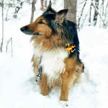
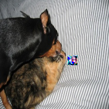
For Patch samples, we trained a autoencoder and used the reconstruction error of $L_{inf}$ distance as a judgment metric. As the patch adversarial examples have a significant noise in a region about 20*20, the reconstruction error tends to be close to 1 for that type of adversarial examples, while the reconstruction error for benign samples is closer to 0.

          

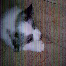
For Square samples, a distinctive feature is the presence of some colored vertical stripes and rectangles visible to the naked eye on the picture. And we noted that the H channel has significant vertical stripes after converting the color space to HSV space. Therefore, we further calculated the difference of the sum of each column. The larger the difference indicates that the corresponding image is more likely to be a Square sample.

          

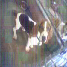
For UAP and FGSM samples, they are characterized by the presence of some noise or continuous texture on the image. To make these features more prominent, we used a Laplacian operator to enhance the edges and subsequently enhance the effect of the noise. Similar to square samples, we observed that the noise in the V channel is more pronounced after transforming the images onto HSV space. To measure the amount of noise, we computed histograms for the V channel. The more the curve on the histograms plot is skewed in the positive direction of the x-axis, the more noisy the image is, and the more likely it is a UAP or FGSM sample. Therefore, we constructed an expression to determine the shape of the histogram curve and subsequently whether the image is an adversarial sample.

         

For other samples, we directly utilize the metrics used for square detection as the organizer will find out the best threshold that yields the highest F1-Score, rather than requiring us to make a binary classification. Our intention was to use the model output or sample robustness to make judgments, just as [2], but unfortunately the organizers of this competition did not provide model information, so these adversarial examples may have poor transferability against our locally trained model.

          

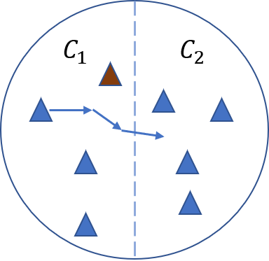
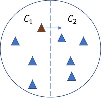
Distance to decision boundary of a blue normal example and brown adversarial example.

Ablation Study

We constructed the dataset locally and evaluated our method.

• For Patch attack, the local F1 score on all adversarial examples is 0.2792, where the precision is 0.9829 and the recall is 0.1627. The F1 score for Patch is 0.9812, where the recall of Patch adv is 0.9795.

• For Square attack, the local F1 score on all adversarial examples is 0.2729, where the precision is 0.932 and the recall is 0.1609. The F1 score for Sqaure is 0.8007, where the recall of Square adv is 0.8614.

• For UAP or FGSM attack, the local F1 score on all adversarial examples is 0.478, where the precision is 0.8483 and the recall is 0.3328. The F1 score for UAP or FGSM is 0.8711, where the recall of UAP or FGSM adv is 0.8951.

Reference

[1] Meng, Dongyu, and Chen, Hao. “Magnet: a two-pronged defense against adversarial examples.” CCS 2017.

[2] Zhao, Zhe, et al. “Attack as defense: characterizing adversarial examples using robustness.” ISSTA 2021.

[3] Karmon, Danny, et al. “LaVAN: Localized and Visible Adversarial Noise.” ICML 2018.

[4] Andriushchenko, Maksym, et al. “Square Attack: A Query-Efficient Black-Box Adversarial Attack via Random Search.” ECCV 2020.

[5] Moosavi-Dezfooli, Seyed-Mohsen, et al. “Universal adversarial perturbations.” arXiv 2016.

[6] Goodfellow, Ian J, et al. “Explaining and harnessing adversarial examples.” arXiv 2014.